Introduction
Every week, someone publishes a single-cell result that is actually a batch artifact. The correction looks convincing on the UMAP. The clusters are clean and neatly separated. The reviewer didn't catch it. Neither did the authors.
This is not a rare failure mode. It is one of the most systematic blind spots in single-cell transcriptomics — and one of the least discussed, because the output looks fine.
Harmony, Seurat, ComBat, scVI... Batch correction tools have become a near-automatic step in scRNA-seq analysis pipelines. They are powerful, well-benchmarked, and, in many situations, genuinely effective. But they share a fundamental limitation that no amount of engineering can overcome: no algorithm can rescue a flawed experimental design. When the technical and biological sources of variation are perfectly intertwined, separation becomes mathematically impossible — not just computationally difficult.
Understanding where this boundary lies is not a minor technical detail. It determines what you can and cannot conclude from your data.
Batch correction is a powerful computational tool, but it only works when biological and technical variability are not perfectly confounded.
What is a batch effect in scRNA-seq?
A batch effect is a systematic technical variation that affects gene expression measurements between groups of samples processed under different conditions.
Common sources include:
- Tissue dissociation — enzymes, incubation time, temperature
- Cell capture — platform, reagent lot, operator
- Library preparation — reverse transcription reagents, PCR cycles
- Sequencing — flowcell, lane, sequencing depth
Compared with bulk RNA-seq, scRNA-seq introduces two additional challenges:
- Cell type composition may vary between batches
- Stochastic dropout introduces substantial cell-level noise that can amplify technical differences
The existence of batch effects is not inherently problematic — they are almost inevitable in practice, and the field has developed robust tools to handle them. The problem arises when they become inseparable from the biological signal of interest.
Consider a realistic scenario: tumor biopsies, which are fragile, are processed 30 minutes faster than matched normal tissue to limit necrosis. As a result, every tumor cell now exhibits a differential stress signature compared to controls. After Harmony, the UMAP looks clean. However, stress response genes — HSPA1A, JUN, FOS — are now associated with tumor status. They will appear in the differential expression table, be included in the paper, and cited by others.
This is not a hypothetical. Variants of this scenario have appeared in the literature repeatedly.
Overview of batch correction methods
The field of batch correction in scRNA-seq has matured significantly over the past decade. These methods operate at different stages of the analysis pipeline and rely on different assumptions. Understanding these differences is essential both for choosing an appropriate approach and for recognizing when none will suffice.
| Method | Approach | Level | Strengths & limitations |
|---|---|---|---|
| Harmony | Iterative soft clustering in PCA space with batch-aware correction | Very fast and robust. Resistant to overcorrection. Often recommended as a first pass. Does not modify the count matrix. | |
| Seurat v4/v5 (CCA/RPCA) | Anchor identification between datasets via CCA or RPCA | Embedding / Matrix | Widely used. May mix distinct cell populations when batch compositions differ substantially. |
| ComBat / ComBat-seq | Empirical Bayesian model applied directly to expression data | Corrected matrix | Statistically well characterized. Performs well in several benchmarks. ComBat-seq preserves count properties. Less suited for non-linear batch effects. |
| scVI | Deep generative model (VAE) modeling counts with a negative binomial distribution in a latent space | Probabilistic modeling of counts. Highly scalable. Integrated differential expression. May overcorrect in certain situations. | |
| scANVI | Semi-supervised extension of scVI using cell annotations | Better preservation of biological signal when reliable labels are available. Useful for label transfer. | |
| MNN / FastMNN | Alignment based on mutual nearest neighbors between batches | Corrected matrix | Elegant concept. Requires shared cell populations between batches. |
| BBKNN | Construction of a batch-balanced KNN graph | KNN graph | Lightweight and fast. Does not modify counts or embeddings, only the neighbor graph structure. |
Benchmarks such as scIB (Luecken et al., 2022, Nature Methods) show that no single method is universally optimal. Harmony and Seurat perform well for straightforward integrations, while scVI or scANVI are often preferred for complex multi-study integrations.
The best choice depends on several factors: the type of batch effect, dataset size, the required output (embedding vs corrected matrix), and the biological question being addressed.
Fundamental limits of batch correction
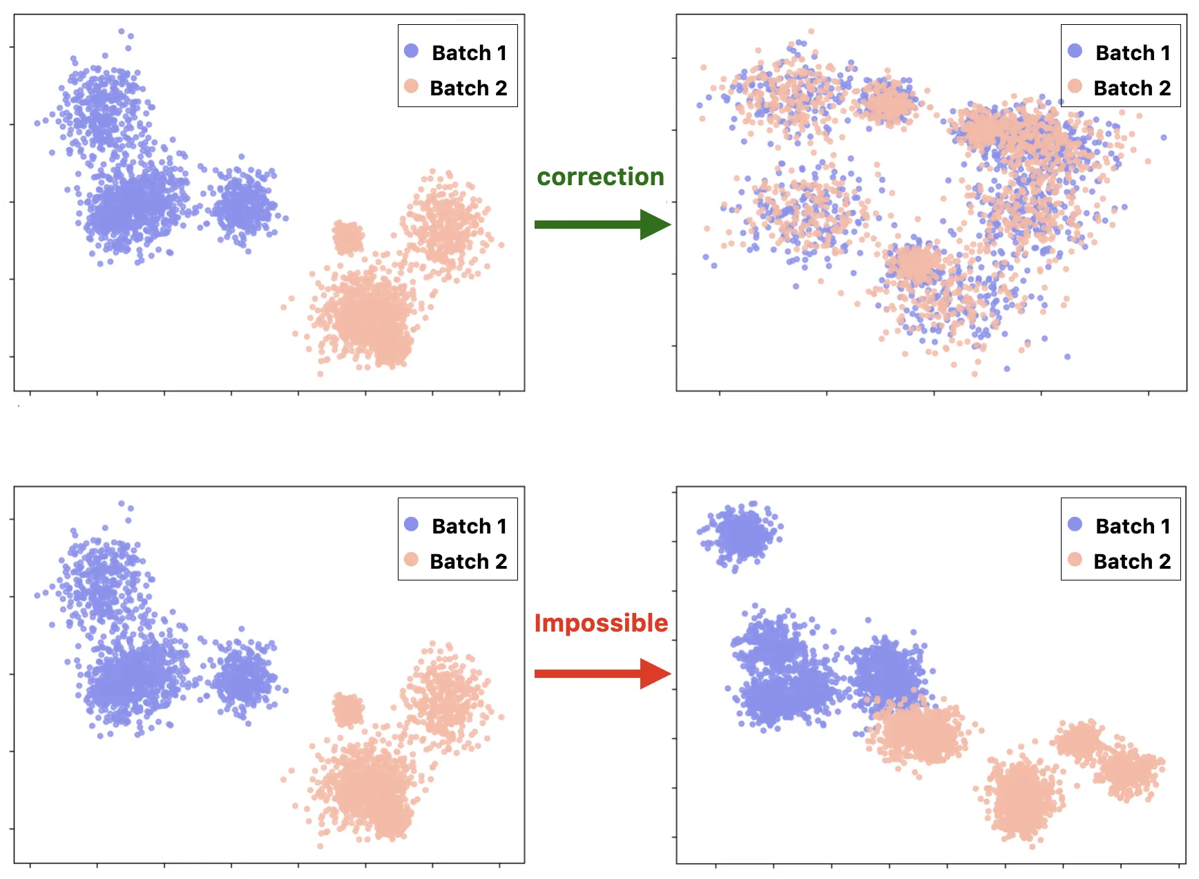
All batch correction methods share a key assumption: biological and technical variability must be statistically separable. When batch and biology are perfectly correlated, reliable correction becomes impossible.
In practice, we encounter this limitation frequently — and it usually has less to do with the choice of algorithm than with decisions made months earlier at the bench.
Confounding: when batch equals biology
Consider a simple example:
- Control cells processed on Monday (batch 1)
- Treated cells processed on Tuesday (batch 2)
In this scenario:
- No correction leaves a technical bias
- Correction risks removing the biological signal of interest
Both options are wrong. There is no third option that makes the problem disappear.
This problem was formally described by Song et al. (2020, Nature Communications), who showed that in a fully confounded design, no method can correctly separate batch and biological effects. They also demonstrated that certain experimental strategies — such as the reference panel design or the chain-type design — allow valid correction precisely because they break the perfect correlation between batch and biology.
The mathematical intuition is straightforward: a linear model cannot simultaneously estimate two variables that are perfectly collinear. What algorithms do in these situations is not correction — it is arbitrary partition of variance between two indistinguishable sources.
If your biological variable of interest (treatment, disease condition, etc.) is perfectly confounded with batch, no computational method — no matter how sophisticated — can separate the two. This is not a software limitation; it is a mathematical impossibility.
Overcorrection: when biology disappears
The opposite problem is overcorrection.
Recent work has shown that many correction methods can alter data more than necessary. Excessive correction may:
- Remove known marker genes
- Merge biologically distinct cell populations
- Artificially reduce the number of differentially expressed genes
Some methods appear more resistant to overcorrection than others. Harmony, for instance, operates locally in PCA space and tends to preserve global structure reasonably well. Deeper generative approaches like scVI are more expressive — which is both their strength and their risk. A model with enough capacity to learn complex batch structures also has enough capacity to learn complex biological structures and erase them.
The problem is that overcorrection often goes undetected. After correction, a UMAP that looks biologically coherent provides no guarantee that the underlying expression matrix still reflects real biology. New evaluation frameworks such as RBET (Ye et al., 2025, Communications Biology) attempt to quantify this using reference gene sets — but these tools are not yet widely integrated into standard pipelines.
What about foundation models?
The emergence of single-cell foundation models — scGPT, Geneformer, Universal Cell Embeddings — has raised hopes for learning universal representations capable of transcending batch effects. The premise is appealing: train on millions of cells across hundreds of studies, and perhaps the model learns to encode cell identity in a space where technical variation is irrelevant.
In practice, the picture is more complicated. When you examine the latent representations of these models, batch structure is often still visible — sometimes attenuated, rarely eliminated. The reason is not a failure of model architecture. It is a more fundamental issue: batch effects are encoded in the training data itself. A model trained on data where "tumor" and "high stress response" co-occur cannot learn to disentangle them, regardless of how many parameters it has.
Integrating batch correction objectives directly into model training is an active area of research. The results so far are promising but preliminary. For now, foundation models are powerful tools for cell type annotation and cross-study comparison — but they do not eliminate the need for careful experimental design, and they do not solve confounded designs.
Peer review does not catch this
This is worth stating directly, because it shapes the incentives of the field.
Reviewers typically see the final UMAP, the cluster annotations, and the differential expression tables. They rarely see the experimental design matrix — the table that would reveal whether any biological condition appears in only one batch. Integration metrics like kBET or LISI are still not routinely reported in publications. And a well-corrected confounded dataset can produce metrics that look perfectly acceptable, because the metrics measure batch mixing, not biological fidelity.
The result is a systematic blind spot. Studies with confounded designs can clear peer review, produce clean visualizations, and generate cited findings — all while reporting what is, in part, a technical artifact. This is not a criticism of individual researchers. It is a structural problem with how single-cell results are currently evaluated and reported.
Experimental design: the first line of defense
The best time to deal with a batch effect is before it exists.
A rigorous experimental design is far more effective than any downstream computational correction. And crucially, the key decisions happen before sequencing — often before any data exists to reveal the problem.
Best practices at the bench
Several strategies help minimize batch effects during experimental preparation:
- Process all samples under identical experimental conditions (same operator, reagent lots, equipment, and timing)
- Randomize sample placement on capture devices
- Use multiplexing approaches to pool biologically different samples within the same technical run
Multiplexing is particularly powerful because it directly breaks the confounding between batch and biology. When treated and control cells are captured together in the same well, any technical variation from that capture step affects both equally.
Experimental designs that enable correction
When multiplexing is not feasible, two experimental strategies have been formally shown to allow valid correction.
The reference panel design includes a shared reference sample in every batch. This common anchor allows estimation and subtraction of batch effects because it provides a biological signal that should be identical across batches — any difference is by definition technical.
The chain-type design ensures that at least one cell population or sample is shared between consecutive batches, creating a chain of biological bridges across the experiment.
Both strategies rely on the same fundamental principle: each batch must share at least one biological component with another batch so that algorithms can distinguish technical variation from biological variation.
Before starting your experiment, construct a simple contingency table of batches × biological conditions. If any condition appears in only one batch, it is a major warning sign. Fix the design now — not after sequencing.
Diagnosing an irrecoverable batch effect
How can you determine whether a batch effect is beyond correction?
Before correction
Start by examining PCA or UMAP colored by batch. If cells cluster primarily by batch rather than expected biological categories, this is an initial warning sign — but not necessarily fatal.
The critical diagnostic is the contingency table of batch versus biological condition. If any cell of this table is zero (a condition that only appears in one batch), you have at minimum a partially confounded design. If every condition appears in only one batch, the design is fully confounded and computational correction cannot help.
After correction
Even when correction appears successful, careful validation is necessary. A UMAP that looks clean after integration is not evidence of successful correction — it is evidence that the algorithm converged. Those are not the same thing.
Check that known marker genes remain properly expressed in the expected populations. Compare differential expression analyses performed with and without correction. A large reduction in the number of DE genes after correction should prompt suspicion: are you removing noise, or signal?
Quantitative metrics can also help:
- kBET — k-nearest-neighbor Batch Effect Test
- LISI — Local Inverse Simpson's Index
- ASW — Average Silhouette Width
- ARI — Adjusted Rand Index
Use these metrics, but interpret them carefully. They measure batch mixing — not biological preservation.
Warning signs of overcorrection
Typical red flags include:
- Ribosomal or mitochondrial genes dominating cluster markers
- Biologically distinct populations merging in the corrected embedding
- Expected rare subpopulations disappearing after correction
- A large drop in the number of differentially expressed genes
- Known positive control marker genes losing cell-type specificity
Checklist before starting your analysis
At the experimental design stage
- Ensure there is no confounding between batch and the biological variable of interest
- Include a reference sample in every batch if multiplexing is not possible
- Standardize protocols (operator, reagents, timing) and document deviations
- Carefully record all technical metadata — reagent lots, dissociation times, operators, capture devices
At the analysis stage
- Visualize data before correction (PCA/UMAP colored by batch and condition)
- Build and examine the batch × condition contingency table
- Try Harmony as a fast first-pass integration method
- Evaluate results using quantitative metrics (kBET, LISI, ARI)
- Validate known canonical marker genes before and after correction
- If necessary, test scVI or Seurat as alternatives
- When cell composition differs strongly between batches, consider scANVI if reliable annotations are available
When correction fails
- Accept the diagnosis — avoid forcing corrections that erase the signal to produce a cleaner-looking UMAP
- Reformulate biological questions based on dataset limitations (e.g., intra-batch analyses, analyses restricted to shared populations)
- If scientifically justified, consider repeating the experiment with an improved design
- Document the limitation transparently in any publication
Conclusion
Modern batch correction methods are powerful, but they rely on one critical assumption: biology and technical variation must be distinguishable. When experimental design is fully confounded, no computational method can recover the lost information. The algorithm will still run. The UMAP will still look clean. The results will still be publishable.
That is precisely what makes this problem dangerous.
If you are planning an experiment, the contingency table is the most important figure you will draw before collecting a single cell. If you are analyzing existing data, a careful diagnostic will at least clarify what the dataset can — and cannot — reliably reveal. The honest answer to that question is more valuable than a polished figure built on an irrecoverable design.
Batch correction tools are powerful — but they cannot rescue a flawed experimental design. A clean UMAP is not a guarantee. Sometimes it is exactly the opposite.
References
- Tran HTN et al. A benchmark of batch-effect correction methods for single-cell RNA sequencing data. Genome Biology 21, 12 (2020).
- Korsunsky I et al. Fast, sensitive and accurate integration of single-cell data with Harmony. Nature Methods 16, 1289–1296 (2019).
- Stuart T et al. Comprehensive Integration of Single-Cell Data. Cell 177, 1888–1902 (2019).
- Haghverdi L et al. Batch effects in single-cell RNA-sequencing data are corrected by matching mutual nearest neighbours. Nature Biotechnology 36, 421–427 (2018).
- Lopez R et al. Deep generative modeling for single-cell transcriptomics. Nature Methods 15, 1053–1058 (2018).
- Xu C et al. Probabilistic harmonization and annotation of single-cell transcriptomics data with deep generative models. Molecular Systems Biology 17, e9620 (2021).
- Luecken MD et al. Benchmarking atlas-level data integration in single-cell genomics. Nature Methods 19, 41–50 (2022).
- Song F et al. Flexible experimental designs for valid single-cell RNA-sequencing experiments allowing batch effects correction. Nature Communications 11, 3274 (2020).
- Antonsson SE & Melsted P. Batch correction methods used in single-cell RNA sequencing analyses are often poorly calibrated. Genome Research 35, 1832–1841 (2025).
- Ye Z et al. Reference-informed evaluation of batch correction for single-cell omics data with overcorrection awareness. Communications Biology 8, 504 (2025).
- Tung PY et al. Batch effects and the effective design of single-cell gene expression studies. Scientific Reports 7, 39921 (2017).
- Luecken MD & Theis FJ. Current best practices in single-cell RNA-seq analysis: a tutorial. Molecular Systems Biology 15, e8746 (2019).
- Andreatta M et al. Semi-supervised integration of single-cell transcriptomics data. Nature Communications 15, 872 (2024).